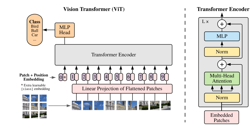
Vision Transformer (ViT)

Reshape the image $ x \in R^{H * W * C}$ into flattened 2D patches $x_{p} \in R^{N * (P^2 C)}$

$(H, W)$ the resolution of original image, $C$ channels, $(P,P)$ resolution for each image patch.

$N=HW / P^2$ the resulting number of patches.

Position Embeddings are added to the patch embeddings to retain positional information.

Inductive bias

ViT has much less image-specific inductive bias than CNNs.

Only MLP layers are local and translationally equivariant, while the self-attention layers are global.

Hybrid Architecture

The input sequence can be formed from feature maps of a CNN.

The patch embedding project is applied to patches from CNN feature map.

Fine-Tuning and Higher Resolution

The paper found that it performs better to fine-tune at higher resolution than pre-training.

The ViT can handle arbitrary sequence lengths but the pre-trained position embeddings may no longer be meaningful.

Point Cloud Transformer PCT

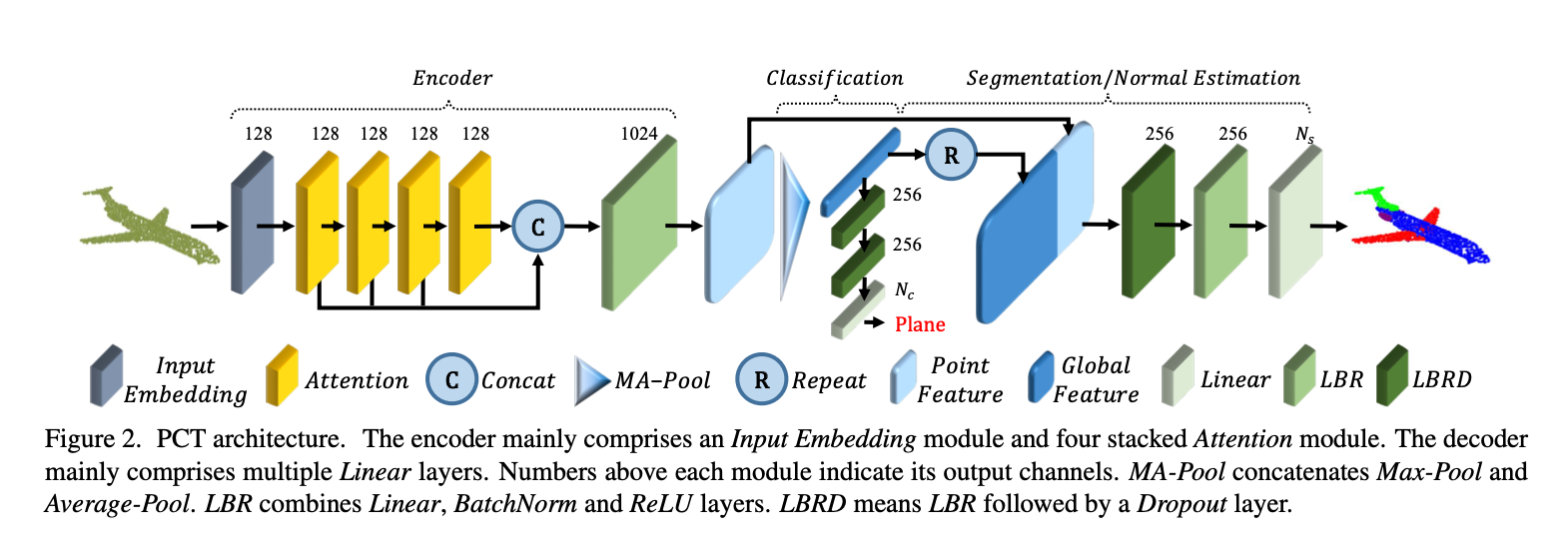
Encoder

1. Embedding the input coordinates into a new feature space.
2. Feed embedded features into 4 stacked attention module.
   • To learn semantically rich and discriminative representation for each point
3. A Linear layer to generate the output feature.

Compared to Ordinary Transformer:

• Share the same philosophy of design
• Positional embedding discarded, because coordinates already contains this info.

Formally:

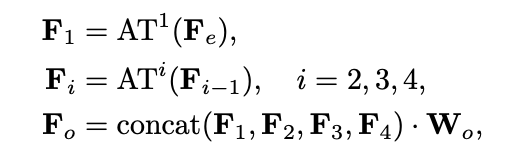
$F_e$ feature embedding for the point clouds.

$AT^i$ $i$_th attention layer.

$W_o$ weight for the linear layer.

Classification

1. Feed global Feature $F_o$ to the classification decoder, consisting two cascaded feed-forward neural networks LBRs (Linear, BatchNorm, and ReLU layers), with dropout rate 0.5.
2. A linear layer to predict the final classification scores $C \in R^{N_c}$ , determined as maximal score.

Segmentation

1. Concatenate global feature $F_g$ with point-wise features in $F_o$.
2. Encode the one-hot object category vector as 64-dim feature and concatenate it with the global feature.
3. dropout only performed on the first LBR.

Normal Estimation

• Same architecture as in segmentation by setting $N=3$, without object category encoding.
• Regard the output point-wise score as the predict normal.

Naive PCT

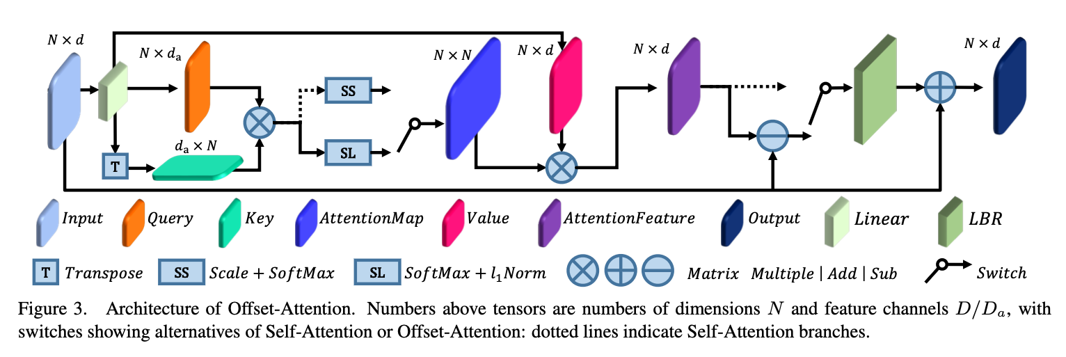
Offset Attention

Replace the Self-Attention module with Offset-Attention Module.

• The OA layer calculates the offset (difference) between the self-attention features and the input features by element-wise subtraction.

Neighbour Embedding

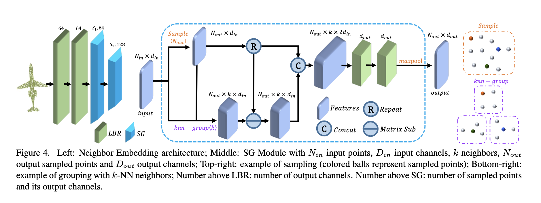
The Neighbour Embedding module contains two LBR layers and two SG (Sampling and grouping) layers.

The SG Layer

• Input point cloud $P$ with $N$ points and corresponding features $F$ , output a sampled point cloud $P_s$ with $N_s$ points and aggregated features $F_s$.

1. Adopt Farthest point sampling (FPS) algorithm to downsample $P \rarr P_s$
2. for each sampled point $p \in P_s$, $knn(p, P)$ is its $k$-nearest neighbours in $P$. The output feature is:

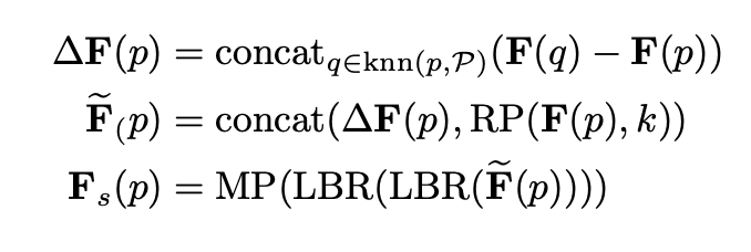
$F(p)$ the input feature of point $p$,

$F_s(p)$ is the output feature of sampled point $p$,

$MP$ is the max-pooling operator,

$RP(x, k)$ repeat vecotr $x$ in $k$ times to form a matrix. (idea from EdgeConv)

---